# Documentation
Here is a list of features loosely organised into those pertaining to
(i) the [`Environment`](#i-environment-features)
* [Adding walls](#walls)
* [Complex Environments: Polygons, curves and holes](#complex-environments-polygons-curves-and-holes)
* [Objects](#objects)
* [Boundary conditions](#boundary-conditions)
* [1- or 2-dimensions](#or-2-dimensions)
(ii) the [`Agent`](#ii-agent-features)
* [Random motion](#random-motion-model)
* [Importing trajectories](#importing-trajectories)
* [Policy control](#policy-control)
* [Wall repelling](#wall-repelling)
* [Multiple Agents](#multiple-agents)
* [Advanced `Agent` classes](#advanced-agent-classes)
(iii) the [`Neurons`](#iii-neurons-features).
* [Cell types](#multiple-cell-types)
* [Noise](#noise)
* [Spikes vs rates](#spiking)
* [Plotting rate maps](#rate-maps)
* [Place cell models](#place-cell-models)
* [Place cell geometry](#geometry-of-placecells)
* [Egocentric encodings](#egocentric-encodings)
* [Reinforcement learning and successor features](#reinforcement-learning-and-successor-features)
* [Deep neural networks](#neurons-as-function-approximators)
* [Create your own `Neuron` types](#creating-your-own-neuron-types)
(iv) [Figures and animations plotting](#iv-figures-and-animations)
Specific details can be found in the [paper](https://www.biorxiv.org/content/10.1101/2022.08.10.503541v3).
## (i) `Environment` features
### **Walls**
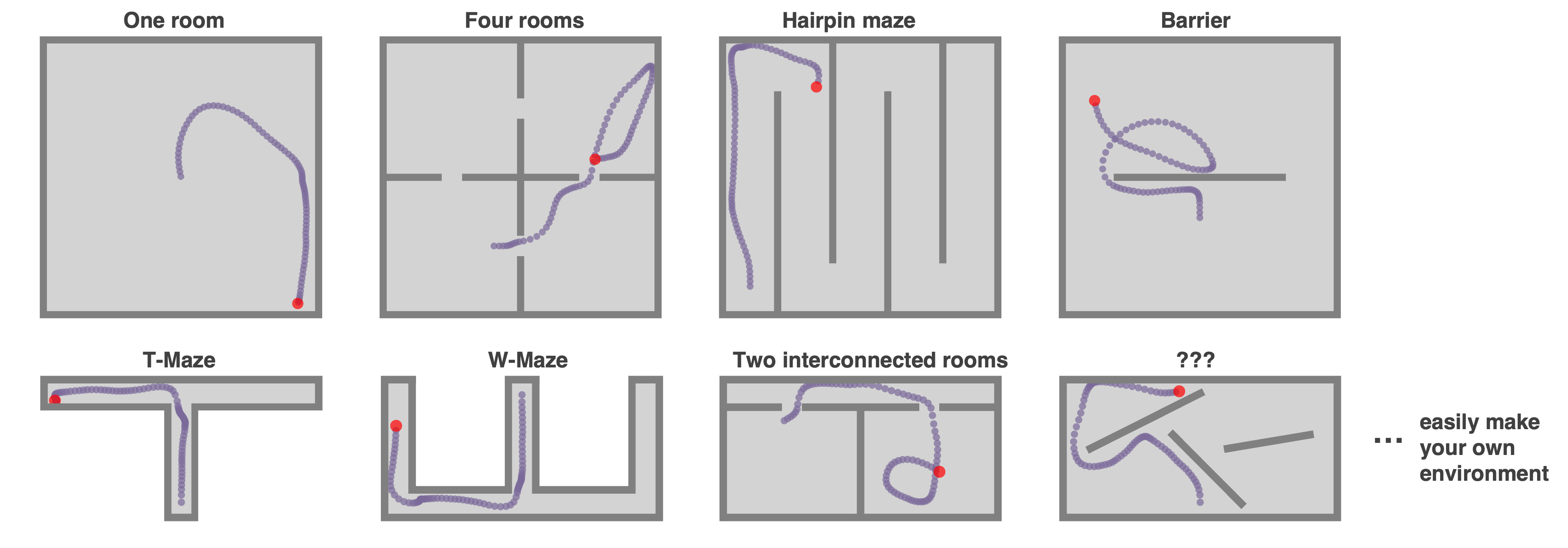
Arbitrarily add walls to the environment to produce arbitrarily complex mazes:
```python
Environment.add_wall([[x0,y0],[x1,y1]])
```
Here are some easy to make examples.
 ### **Complex `Environment`s: Polygons, curves, and holes**
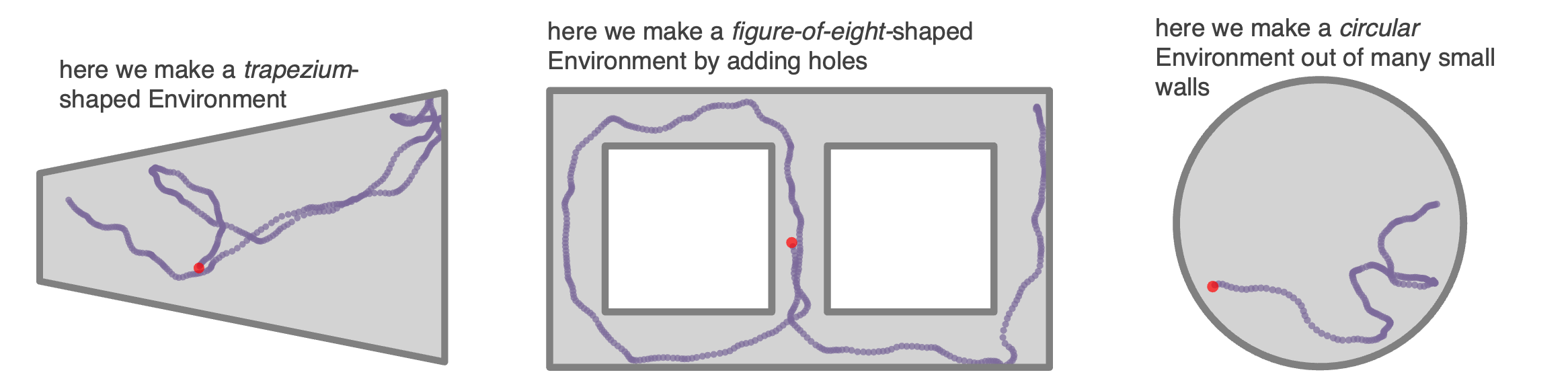
By default, `Environments` in RatInABox are square (or rectangular if `aspect != 1`). It is possible to create arbitrary environment shapes using the `"boundary"` parameter at initialisation.
One can all add holes to the `Environment` using the `"holes"` parameter at initialisation. Positions sampled from the Environment (e.g. at initialisation) won't be inside holes.
Any curved environments can be made by creating a boundary of many small walls (uyse sparingly, walls may slow down computations)
```python
#A trapezium shaped Environment
Env = Environment(params={
'boundary':[[0,-0.2],[0,0.2],[1.5,0.5],[1.5,-0.5]],
})
#An environment with two holes making a figure of 8
Env = Environment(params={
'aspect':1.8,
'holes' : [[[0.2,0.2],[0.8,0.2],[0.8,0.8],[0.2,0.8]],
[[1,0.2],[1.6,0.2],[1.6,0.8],[1,0.8]]],
})
#A circular environment made from many small walls
Env = Environment(params = {
'boundary':[[0.5*np.cos(t),0.5*np.sin(t)] for t in np.linspace(0,2*np.pi,100)],
})
```
### **Complex `Environment`s: Polygons, curves, and holes**
By default, `Environments` in RatInABox are square (or rectangular if `aspect != 1`). It is possible to create arbitrary environment shapes using the `"boundary"` parameter at initialisation.
One can all add holes to the `Environment` using the `"holes"` parameter at initialisation. Positions sampled from the Environment (e.g. at initialisation) won't be inside holes.
Any curved environments can be made by creating a boundary of many small walls (uyse sparingly, walls may slow down computations)
```python
#A trapezium shaped Environment
Env = Environment(params={
'boundary':[[0,-0.2],[0,0.2],[1.5,0.5],[1.5,-0.5]],
})
#An environment with two holes making a figure of 8
Env = Environment(params={
'aspect':1.8,
'holes' : [[[0.2,0.2],[0.8,0.2],[0.8,0.8],[0.2,0.8]],
[[1,0.2],[1.6,0.2],[1.6,0.8],[1,0.8]]],
})
#A circular environment made from many small walls
Env = Environment(params = {
'boundary':[[0.5*np.cos(t),0.5*np.sin(t)] for t in np.linspace(0,2*np.pi,100)],
})
```
 ### **Objects**
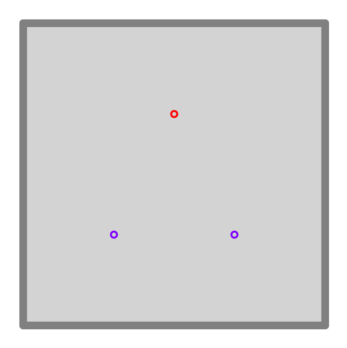
`Environment`s can contain objects. These are used by `ObjectVectorCells` as visual cues but in theory you can hijack these to respresent many things in your `Environment` (reward ports, goal locations etc.). Objects have a `type` and a `position`
Objects are defined by a list of points and a position. Objects can be used as visual cues (e.g. for `ObjectVectorCells`) or as obstacles (e.g. for `BoundaryVectorCells`).
```python
Envirnoment.add_object(object=[0.3,0.3],type=0)
Envirnoment.add_object(object=[0.7,0.3],type=0)
Envirnoment.add_object(object=[0.5,0.7],type=1)
```
### **Objects**
`Environment`s can contain objects. These are used by `ObjectVectorCells` as visual cues but in theory you can hijack these to respresent many things in your `Environment` (reward ports, goal locations etc.). Objects have a `type` and a `position`
Objects are defined by a list of points and a position. Objects can be used as visual cues (e.g. for `ObjectVectorCells`) or as obstacles (e.g. for `BoundaryVectorCells`).
```python
Envirnoment.add_object(object=[0.3,0.3],type=0)
Envirnoment.add_object(object=[0.7,0.3],type=0)
Envirnoment.add_object(object=[0.5,0.7],type=1)
```
 ### **Boundary conditions**
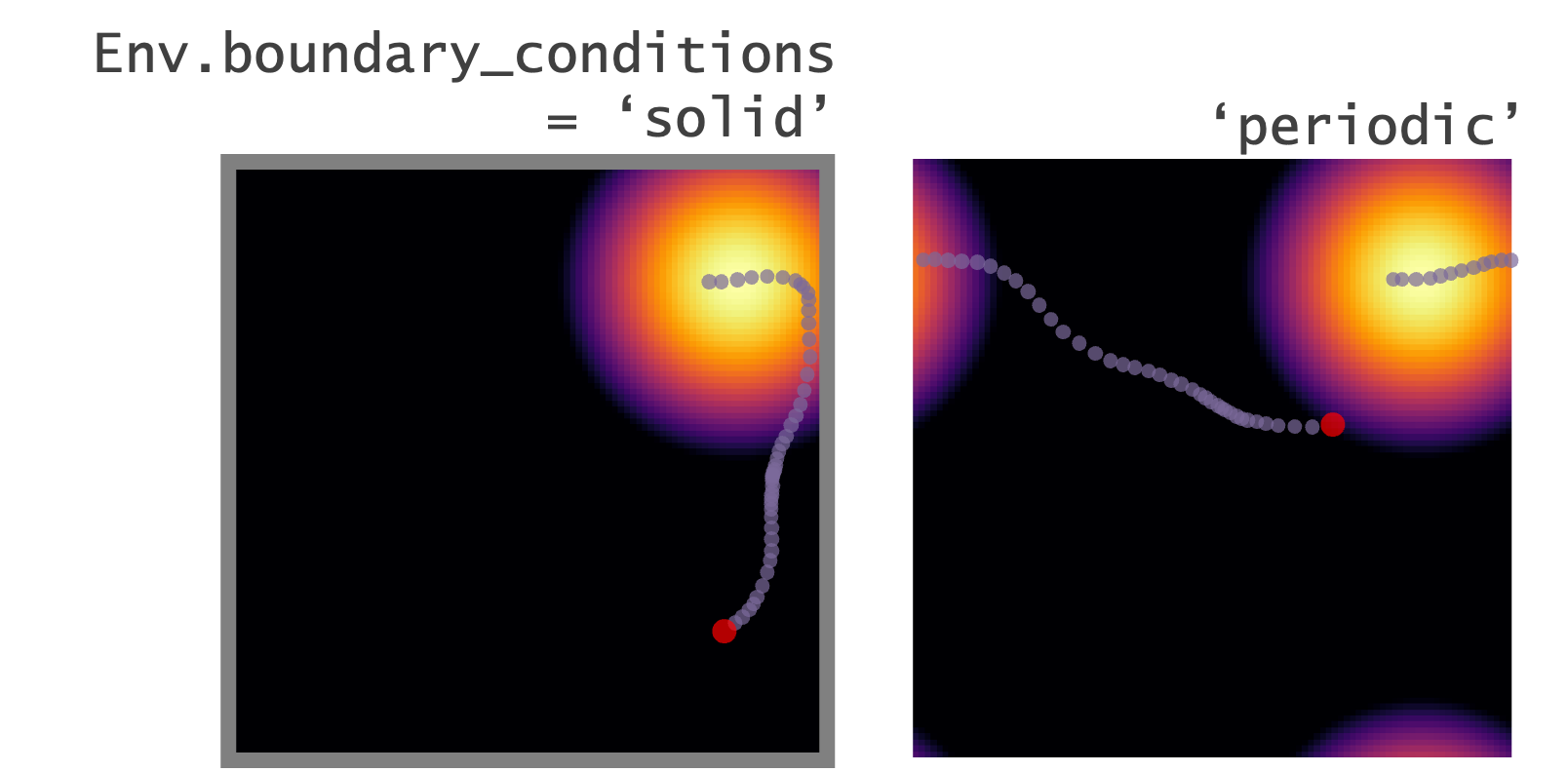
Boundary conditions (for default square/rectangular environments) can be "periodic" or "solid". Place cells and the motion of the Agent will respect these boundaries accordingly.
```python
Env = Environment(
params = {'boundary_conditions':'periodic'} #or 'solid' (default)
)
```
### **Boundary conditions**
Boundary conditions (for default square/rectangular environments) can be "periodic" or "solid". Place cells and the motion of the Agent will respect these boundaries accordingly.
```python
Env = Environment(
params = {'boundary_conditions':'periodic'} #or 'solid' (default)
)
```
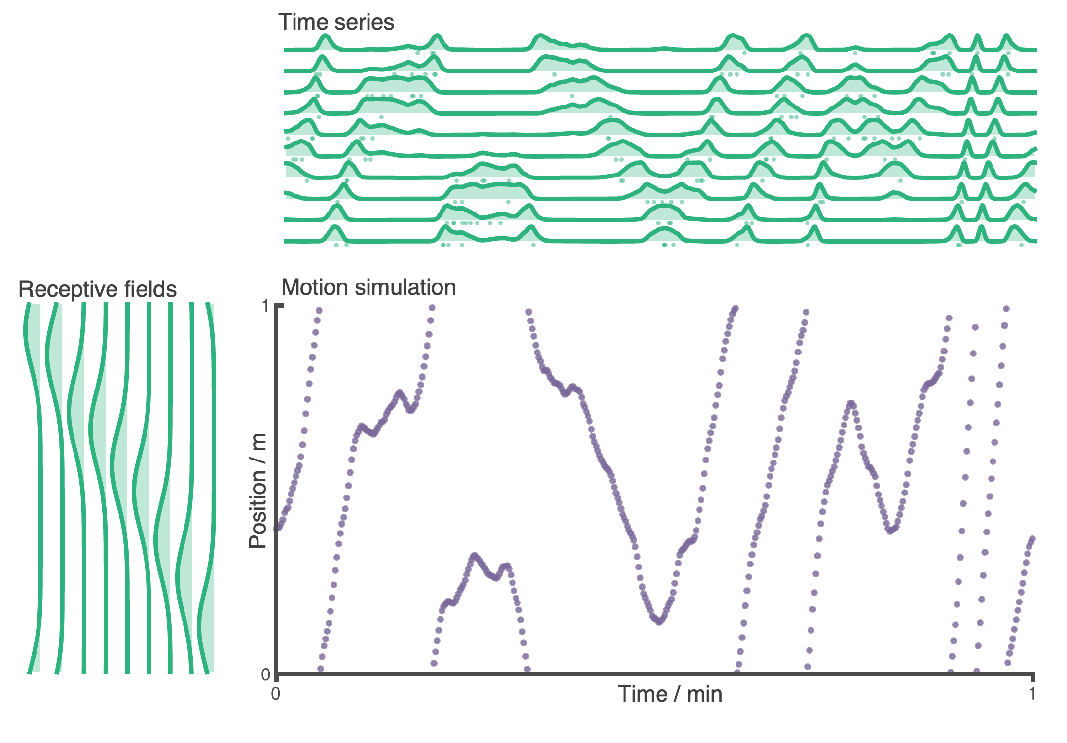
 ### **1--or-2-dimensions**
`RatInABox` supports 1- or 2-dimensional `Environment`s. Almost all applicable features and plotting functions work in both. The following figure shows 1 minute of exploration of an `Agent` in a 1D environment with periodic boundary conditions spanned by 10 place cells.
```python
Env = Environment(
params = {'dimensionality':'1D'} #or '2D' (default)
)
```
### **1--or-2-dimensions**
`RatInABox` supports 1- or 2-dimensional `Environment`s. Almost all applicable features and plotting functions work in both. The following figure shows 1 minute of exploration of an `Agent` in a 1D environment with periodic boundary conditions spanned by 10 place cells.
```python
Env = Environment(
params = {'dimensionality':'1D'} #or '2D' (default)
)
```
 ## (ii) `Agent` features
### **Random motion model**
By defaut the `Agent` follows a random motion policy. Random motion is stochastic but smooth. The speed (and rotational speed, if in 2D) of an Agent take constrained random walks governed by Ornstein-Uhlenbeck processes. You can change the means, variance and coherence times of these processes to control the shape of the trajectory. Default parameters are fit to real rat locomotion data from Sargolini et al. (2006):
## (ii) `Agent` features
### **Random motion model**
By defaut the `Agent` follows a random motion policy. Random motion is stochastic but smooth. The speed (and rotational speed, if in 2D) of an Agent take constrained random walks governed by Ornstein-Uhlenbeck processes. You can change the means, variance and coherence times of these processes to control the shape of the trajectory. Default parameters are fit to real rat locomotion data from Sargolini et al. (2006):
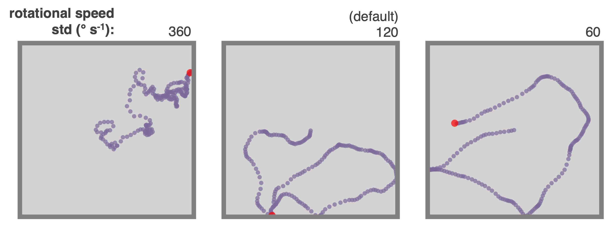
 The default parameters can be changed to obtain different style trajectories. The following set of trajectories were generated by modifying the rotational speed parameter `Agent.rotational_velocity_std`:
```python
Agent.speed_mean = 0.08 #m/s
Agent.speed_coherence_time = 0.7
Agent.rotation_velocity_std = 120 * np.pi/180 #radians
Agent.rotational_velocity_coherence_time = 0.08
```
The default parameters can be changed to obtain different style trajectories. The following set of trajectories were generated by modifying the rotational speed parameter `Agent.rotational_velocity_std`:
```python
Agent.speed_mean = 0.08 #m/s
Agent.speed_coherence_time = 0.7
Agent.rotation_velocity_std = 120 * np.pi/180 #radians
Agent.rotational_velocity_coherence_time = 0.08
```
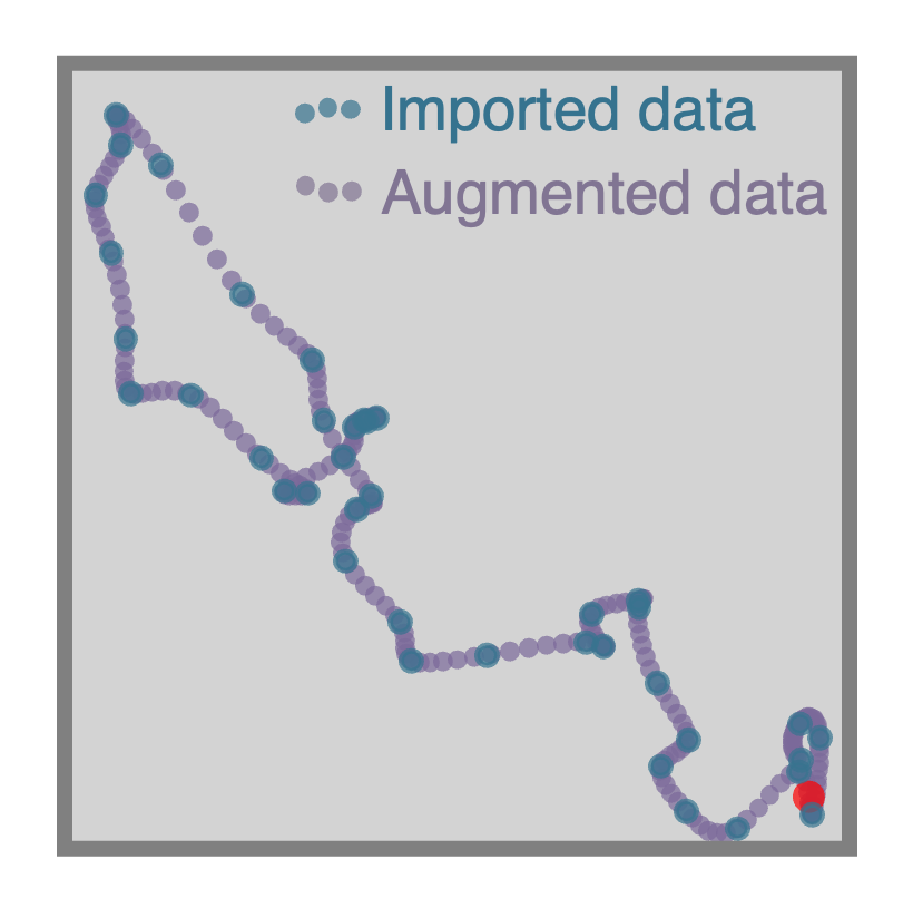
 ### **Importing trajectories**
`RatInABox` supports importing external trajectory data (rather than using the in built random motion policy). Imported data can be of low temporal resolution. It will be smoothly upsampled using a cubic splines interpolation technique. We provide a 10 minute trajectory from the open-source data set of Sargolini et al. (2006) ready to import. In the following figure blue shows (low resolution) trajectory data imported into an `Agent` and purple shows the smoothly upsampled trajectory taken by the `Agent` during exploration.
```python
Agent.import_trajectory(dataset='sargolini')
#or
Agent.import_trajectory(times=array_of_times,
positions=array_of_positions)
```
### **Importing trajectories**
`RatInABox` supports importing external trajectory data (rather than using the in built random motion policy). Imported data can be of low temporal resolution. It will be smoothly upsampled using a cubic splines interpolation technique. We provide a 10 minute trajectory from the open-source data set of Sargolini et al. (2006) ready to import. In the following figure blue shows (low resolution) trajectory data imported into an `Agent` and purple shows the smoothly upsampled trajectory taken by the `Agent` during exploration.
```python
Agent.import_trajectory(dataset='sargolini')
#or
Agent.import_trajectory(times=array_of_times,
positions=array_of_positions)
```
 ### **Policy control**
By default the movement policy is an random and uncontrolled (e.g. displayed above). It is possible, however, to manually pass a "drift_velocity" to the Agent on each `Agent.update()` step. This 'closes the loop' allowing, for example, Actor-Critic systems to control the Agent policy. As a demonstration that this method can be used to control the agent's movement we set a radial drift velocity to encourage circular motion. We also use RatInABox to perform a simple model-free RL task and find a reward hidden behind a wall (the full script is given as an example script [here](https://github.com/RatInABox-Lab/RatInABox/blob/main/demos/reinforcement_learning_example.ipynb))
```python
Agent.update(drift_velocity=drift_velocity)
```
### **Policy control**
By default the movement policy is an random and uncontrolled (e.g. displayed above). It is possible, however, to manually pass a "drift_velocity" to the Agent on each `Agent.update()` step. This 'closes the loop' allowing, for example, Actor-Critic systems to control the Agent policy. As a demonstration that this method can be used to control the agent's movement we set a radial drift velocity to encourage circular motion. We also use RatInABox to perform a simple model-free RL task and find a reward hidden behind a wall (the full script is given as an example script [here](https://github.com/RatInABox-Lab/RatInABox/blob/main/demos/reinforcement_learning_example.ipynb))
```python
Agent.update(drift_velocity=drift_velocity)
```
 ### **Wall repelling**
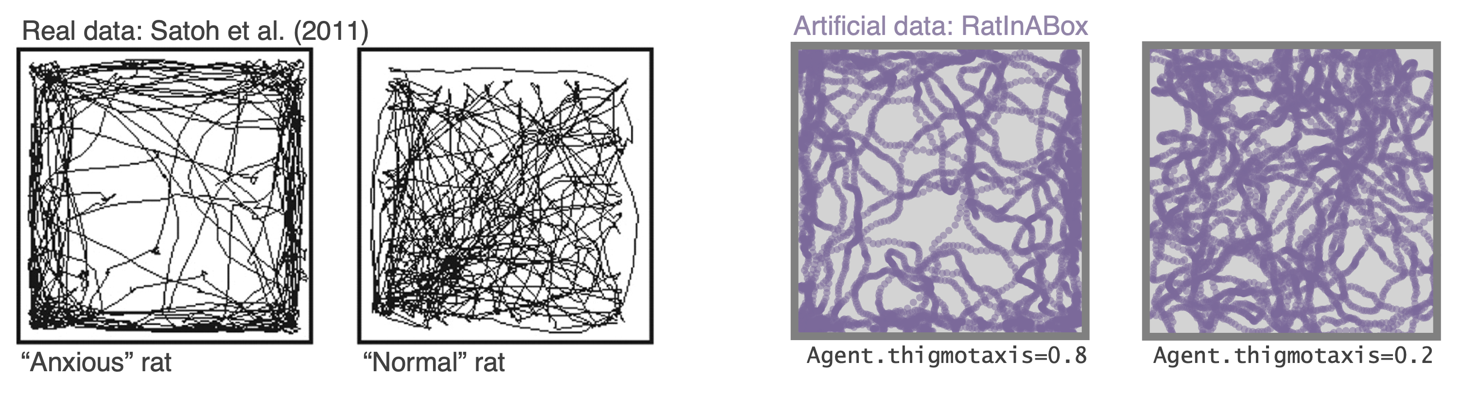
Under the random motion policy, walls in the environment mildly "repel" the `Agent`. Coupled with the finite turning speed this replicates an effect (known as thigmotaxis, sometimes linked to anxiety) where the `Agent` is biased to over-explore near walls and corners (as shown in these heatmaps) matching real rodent behaviour. It can be turned up or down with the `thigmotaxis` parameter.
```python
Αgent.thigmotaxis = 0.8 #1 = high thigmotaxis (left plot), 0 = low (right)
```
### **Wall repelling**
Under the random motion policy, walls in the environment mildly "repel" the `Agent`. Coupled with the finite turning speed this replicates an effect (known as thigmotaxis, sometimes linked to anxiety) where the `Agent` is biased to over-explore near walls and corners (as shown in these heatmaps) matching real rodent behaviour. It can be turned up or down with the `thigmotaxis` parameter.
```python
Αgent.thigmotaxis = 0.8 #1 = high thigmotaxis (left plot), 0 = low (right)
```
 ### **Multiple `Agent`s**
There is nothing to stop multiple `Agent`s being added to the same `Environment`. When plotting/animating trajectories set the kwarg `plot_all_agents=True` to visualise all `Agent`s simultaneously.
The following animation shows three `Agent`s in an `Environment`. Drift velocities are set so that `Agent`s weally locally attract one another creating "interactive" behaviour.
### **Multiple `Agent`s**
There is nothing to stop multiple `Agent`s being added to the same `Environment`. When plotting/animating trajectories set the kwarg `plot_all_agents=True` to visualise all `Agent`s simultaneously.
The following animation shows three `Agent`s in an `Environment`. Drift velocities are set so that `Agent`s weally locally attract one another creating "interactive" behaviour.
 ### **Advanced `Agent` classes**
One can make more advanced Agent classes, for example `ThetaSequenceAgent()` where the position "sweeps" (blue) over the position of an underlying true (regular) `Agent()` (purple), highly reminiscent of theta sequences observed when one decodes position from the hippocampal populaton code on sub-theta (10 Hz) timescales. This class can be found in the [`contribs`](https://github.com/RatInABox-Lab/RatInABox/tree/main/ratinabox/contribs) directory.
### **Advanced `Agent` classes**
One can make more advanced Agent classes, for example `ThetaSequenceAgent()` where the position "sweeps" (blue) over the position of an underlying true (regular) `Agent()` (purple), highly reminiscent of theta sequences observed when one decodes position from the hippocampal populaton code on sub-theta (10 Hz) timescales. This class can be found in the [`contribs`](https://github.com/RatInABox-Lab/RatInABox/tree/main/ratinabox/contribs) directory.
 ## (iii) `Neurons` features
### **Multiple cell types:**
We provide a list of premade `Neurons` subclasses. These include (but are not limited to):
* `PlaceCells`
* `GridCells`
* `BoundaryVectorCells` (can be egocentric or allocentric)
* `ObjectVectorCells` (can be used as visual cues, i.e. only fire when `Agent` is looking towards them) (can be egocentric or allocentric)
* `HeadDirectionCells`
* `VelocityCells`
* `SpeedCells`
* `RandomSpatialNeurons` - smooth but random spatially tuned neurons
* `FeedForwardLayer` - calculates activated weighted sum of inputs from a provide list of input `Neurons` layers.
* `FieldOfViewNeurons` - Egocentric encoding of what the `Agent` can see
* `NeuralNetworkNeurons` - Maps inputs from a user provided list of input `Neurons` through a user-provided `pytorch` neural network. Can be used to create arbitrary and learnable representations.
`FeedForwardLayer` and `NeuralNetworkNeurons` deserves special mention. Instead of its firing rate being determined explicitly by the state of the `Agent` it summates synaptic inputs from a provided list of input layers (which can be any `Neurons` subclass). This layer is the building block for how more complex networks can be studied using `RatInABox`. `NeuralNetworkNeurons` is the same except instead of linearly summating it passes inputs through any arbitrary deep neural network.
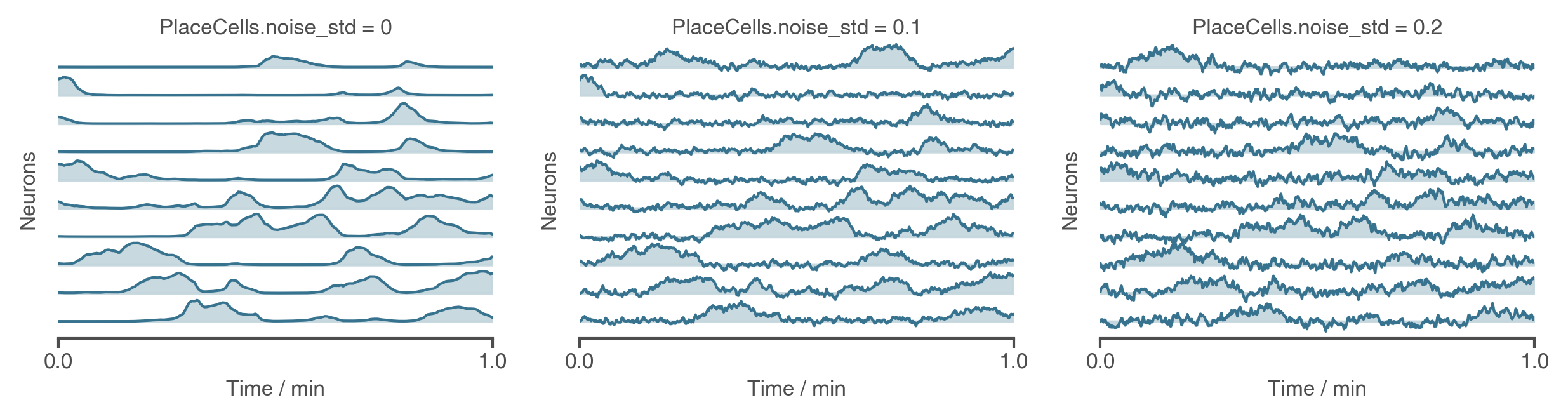
### **Noise**
Use the `Neurons.noise_std` and `Neurons.noise_coherence_time` parameters to control the amount of noise (Hz) and autocorrelation timescale of the noise (seconds). For example (work with all `Neurons` classes, not just `PlaceCells`):
```python
PCs = PlaceCells(Ag,params={
'noise_std':0.1, #defaults to 0 i.e. no noise
'noise_coherence_time':0.5, #autocorrelation timescale of additive noise vector
})
```
## (iii) `Neurons` features
### **Multiple cell types:**
We provide a list of premade `Neurons` subclasses. These include (but are not limited to):
* `PlaceCells`
* `GridCells`
* `BoundaryVectorCells` (can be egocentric or allocentric)
* `ObjectVectorCells` (can be used as visual cues, i.e. only fire when `Agent` is looking towards them) (can be egocentric or allocentric)
* `HeadDirectionCells`
* `VelocityCells`
* `SpeedCells`
* `RandomSpatialNeurons` - smooth but random spatially tuned neurons
* `FeedForwardLayer` - calculates activated weighted sum of inputs from a provide list of input `Neurons` layers.
* `FieldOfViewNeurons` - Egocentric encoding of what the `Agent` can see
* `NeuralNetworkNeurons` - Maps inputs from a user provided list of input `Neurons` through a user-provided `pytorch` neural network. Can be used to create arbitrary and learnable representations.
`FeedForwardLayer` and `NeuralNetworkNeurons` deserves special mention. Instead of its firing rate being determined explicitly by the state of the `Agent` it summates synaptic inputs from a provided list of input layers (which can be any `Neurons` subclass). This layer is the building block for how more complex networks can be studied using `RatInABox`. `NeuralNetworkNeurons` is the same except instead of linearly summating it passes inputs through any arbitrary deep neural network.
### **Noise**
Use the `Neurons.noise_std` and `Neurons.noise_coherence_time` parameters to control the amount of noise (Hz) and autocorrelation timescale of the noise (seconds). For example (work with all `Neurons` classes, not just `PlaceCells`):
```python
PCs = PlaceCells(Ag,params={
'noise_std':0.1, #defaults to 0 i.e. no noise
'noise_coherence_time':0.5, #autocorrelation timescale of additive noise vector
})
```
 ### Spiking
All neurons are rate based. However, at each update spikes are sampled as though neurons were Poisson neurons. These are stored in `Neurons.history['spikes']`. The max and min firing rates can be set with `Neurons.max_fr` and `Neurons.min_fr`.
```
Neurons.plot_ratemap(spikes=True)
```
### Spiking
All neurons are rate based. However, at each update spikes are sampled as though neurons were Poisson neurons. These are stored in `Neurons.history['spikes']`. The max and min firing rates can be set with `Neurons.max_fr` and `Neurons.min_fr`.
```
Neurons.plot_ratemap(spikes=True)
```
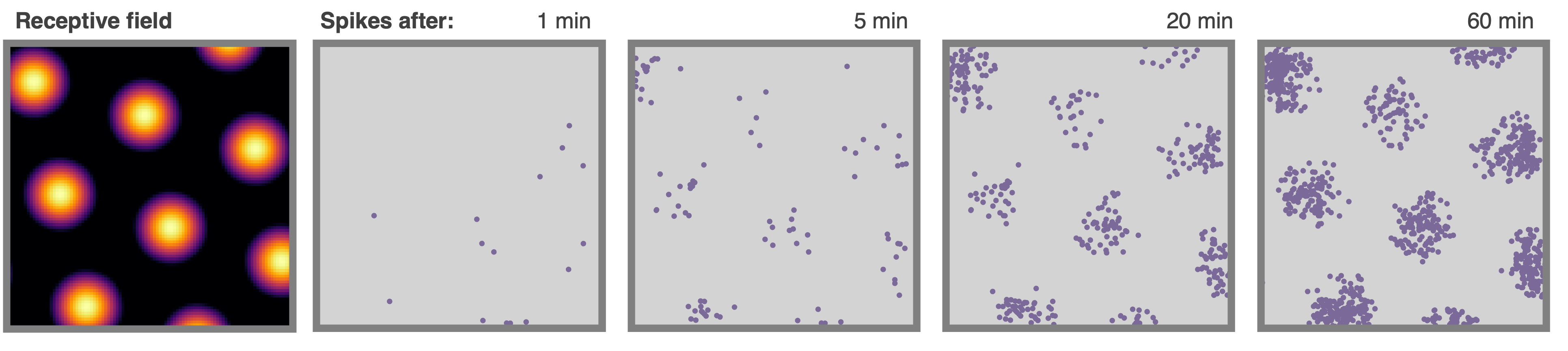 ### **Rate maps**
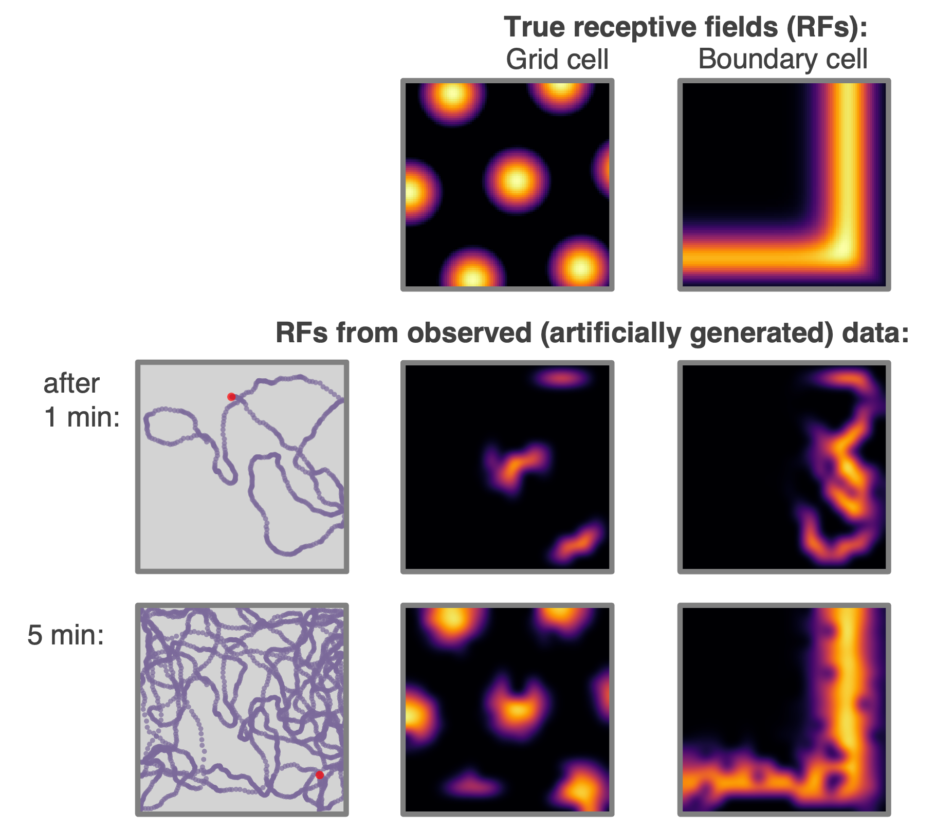
`PlaceCells`, `GridCells` and allocentric `BoundaryVectorCells` (among others) have firing rates which depend exclusively on the position of the agent. These rate maps can be displayed by querying their firing rate at an array of positions spanning the environment, then plotting. This process is done for you using the function `Neurons.plot_rate_map()`.
More generally, however, cells firing is not only determined by position but potentially other factors (e.g. velocity, or historical effects if the layer is part of a recurrent network). In these cases the above method of plotting rate maps will necessarily fail. A more robust way to display the receptive field is to plot a heatmap of the positions of the Agent has visited where each positions contribution to a bin is weighted by the firing rate observed at that position. Over time, as coverage become complete, the firing fields become visible.
```
Neurons.plot_rate_map() #attempts to plot "ground truth" rate map
Neurons.plot_rate_map(method="history") #plots rate map by firing-rate-weighted position heatmap
```
### **Rate maps**
`PlaceCells`, `GridCells` and allocentric `BoundaryVectorCells` (among others) have firing rates which depend exclusively on the position of the agent. These rate maps can be displayed by querying their firing rate at an array of positions spanning the environment, then plotting. This process is done for you using the function `Neurons.plot_rate_map()`.
More generally, however, cells firing is not only determined by position but potentially other factors (e.g. velocity, or historical effects if the layer is part of a recurrent network). In these cases the above method of plotting rate maps will necessarily fail. A more robust way to display the receptive field is to plot a heatmap of the positions of the Agent has visited where each positions contribution to a bin is weighted by the firing rate observed at that position. Over time, as coverage become complete, the firing fields become visible.
```
Neurons.plot_rate_map() #attempts to plot "ground truth" rate map
Neurons.plot_rate_map(method="history") #plots rate map by firing-rate-weighted position heatmap
```
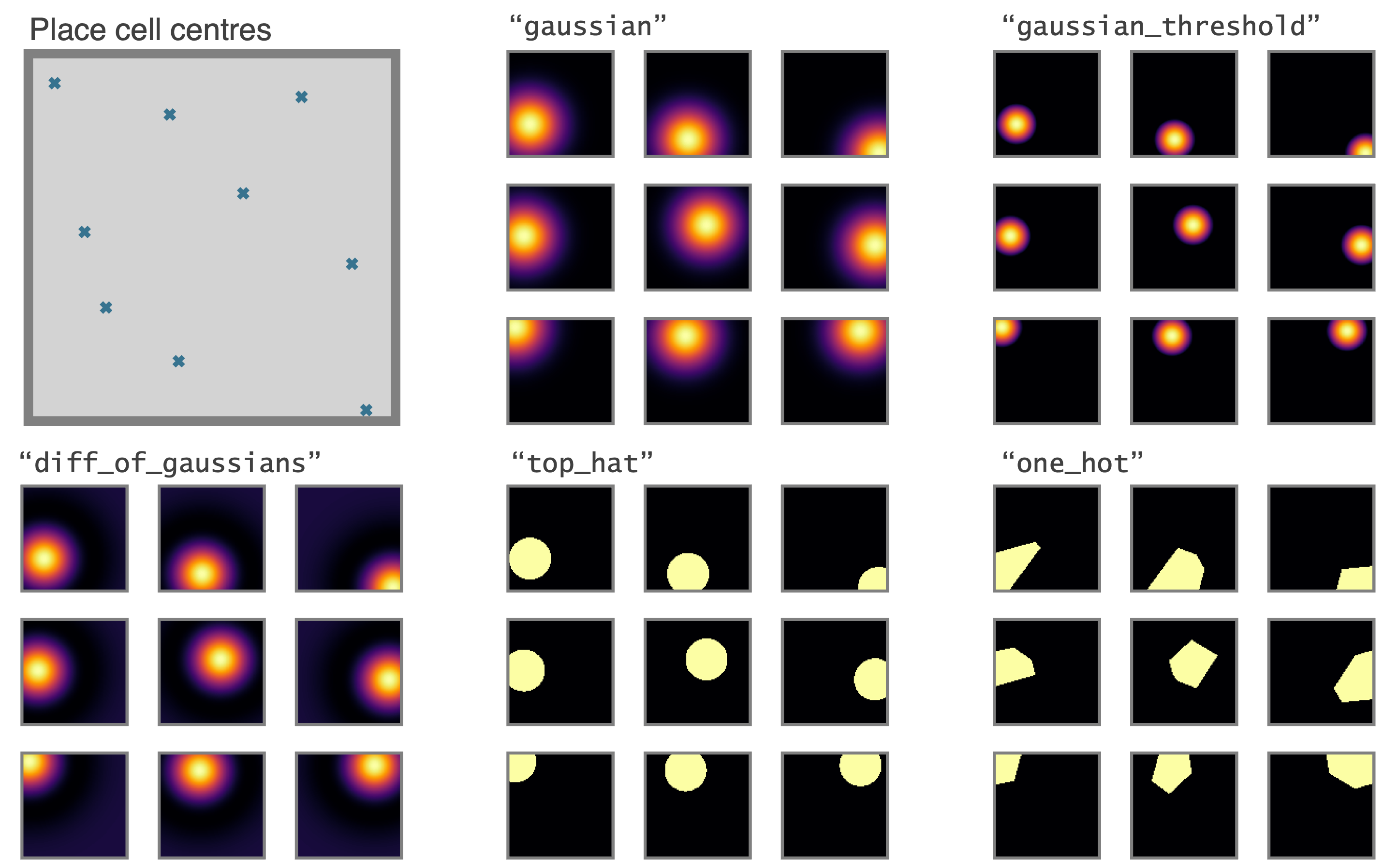
 ### **Place cell models**
Place cells come in multiple types (given by `params['description']`), or it would be easy to write your own:
* `"gaussian"`: normal gaussian place cell
* `"gaussian_threshold"`: gaussian thresholded at 1 sigma
* `"diff_of_gaussians"`: gaussian(sigma) - gaussian(1.5 sigma)
* `"top_hat"`: circular receptive field, max firing rate within, min firing rate otherwise
* `"one_hot"`: the closest place cell to any given location is established. This and only this cell fires.
This last place cell type, `"one_hot"` is particularly useful as it essentially rediscretises space and tabularises the state space (gridworld again). This can be used to contrast and compare learning algorithms acting over continuous vs discrete state spaces. This figure compares the 5 place cell models for population of 9 place cells (top left shows centres of place cells, and in all cases the `"widths"` parameters is set to 0.2 m, or irrelevant in the case of `"one_hot"`s)
### **Place cell models**
Place cells come in multiple types (given by `params['description']`), or it would be easy to write your own:
* `"gaussian"`: normal gaussian place cell
* `"gaussian_threshold"`: gaussian thresholded at 1 sigma
* `"diff_of_gaussians"`: gaussian(sigma) - gaussian(1.5 sigma)
* `"top_hat"`: circular receptive field, max firing rate within, min firing rate otherwise
* `"one_hot"`: the closest place cell to any given location is established. This and only this cell fires.
This last place cell type, `"one_hot"` is particularly useful as it essentially rediscretises space and tabularises the state space (gridworld again). This can be used to contrast and compare learning algorithms acting over continuous vs discrete state spaces. This figure compares the 5 place cell models for population of 9 place cells (top left shows centres of place cells, and in all cases the `"widths"` parameters is set to 0.2 m, or irrelevant in the case of `"one_hot"`s)
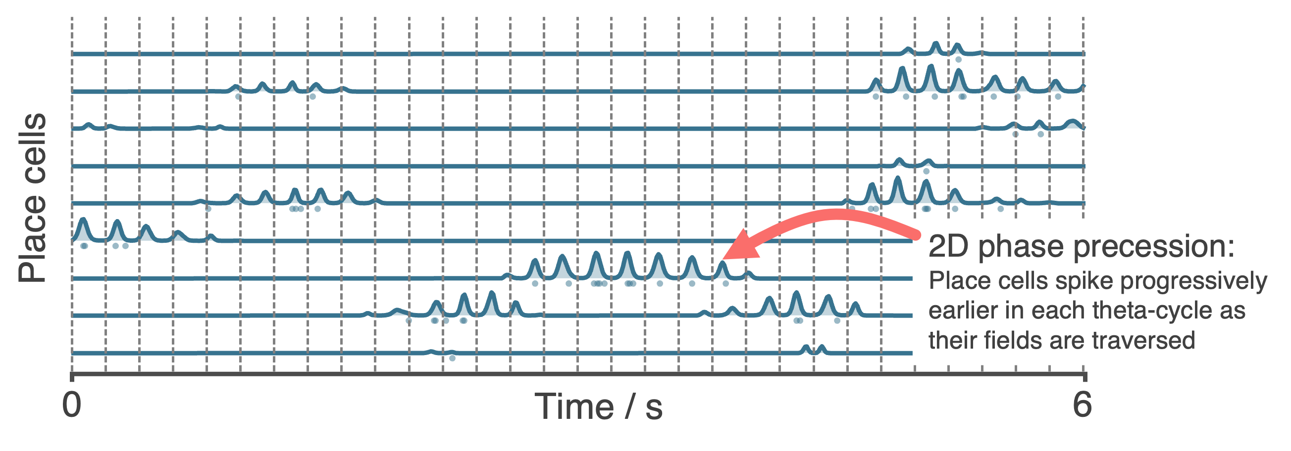
 These place cells (with the exception of `"one_hot"`s) can all be made to phase precess by instead initialising them with the `PhasePrecessingPlaceCells()` class currently residing in the `contribs` folder. This figure shows example output data.
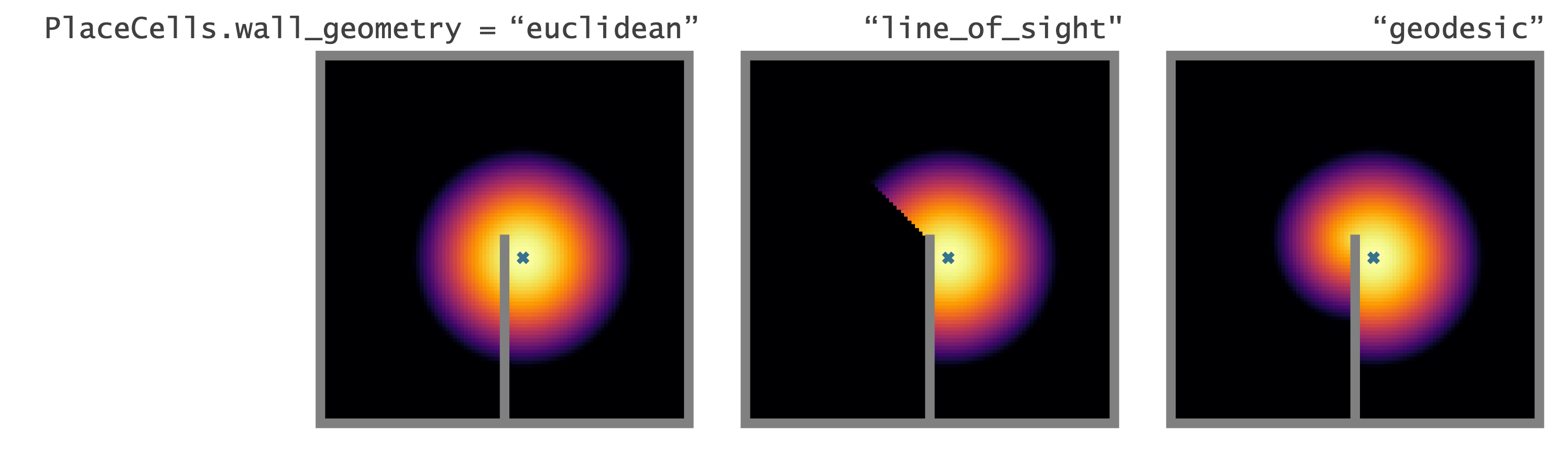
 ### **Geometry of `PlaceCells`**
Choose how you want `PlaceCells` to interact with walls in the `Environment`. We provide three types of geometries.
### **Geometry of `PlaceCells`**
Choose how you want `PlaceCells` to interact with walls in the `Environment`. We provide three types of geometries.
 ### **Egocentric encodings**
Most `RatInABox` cell classes are allocentric (e.g. `PlaceCells`, `GridCells` etc. do not depend on the agents point of view) not egocentric. `BoundaryVectorCells` (BVCs) and `ObjectVectorCells` (OVCs) can be either. `FieldOfViewNeurons` exploit this by arranging sets of egocentric BVC or OVCs to tile to agents local field of view creating a comprehensive egocentric encoding of what boundaries or objects the agent can 'see' from it's current point of view. A custom plotting function displays the tiling and the firing rates as shown below. With an adequately defined field of view these can make, for example, "whisker cells".
```python
FoV_BVCs = FieldOfViewBVCs(Ag)
FoV_OVCs = FieldOfViewOVCs(Ag)
BVCs_whiskers = FieldOfViewBVCs(Ag,params={
"distance_range": [0.01, 0.2],
"angle_range": [
75,
105,
],
"spatial_resolution": 0.02, # resolution of each OVC tiling FoV
"cell_arrangement": "uniform_manifold",
})
```
### **Egocentric encodings**
Most `RatInABox` cell classes are allocentric (e.g. `PlaceCells`, `GridCells` etc. do not depend on the agents point of view) not egocentric. `BoundaryVectorCells` (BVCs) and `ObjectVectorCells` (OVCs) can be either. `FieldOfViewNeurons` exploit this by arranging sets of egocentric BVC or OVCs to tile to agents local field of view creating a comprehensive egocentric encoding of what boundaries or objects the agent can 'see' from it's current point of view. A custom plotting function displays the tiling and the firing rates as shown below. With an adequately defined field of view these can make, for example, "whisker cells".
```python
FoV_BVCs = FieldOfViewBVCs(Ag)
FoV_OVCs = FieldOfViewOVCs(Ag)
BVCs_whiskers = FieldOfViewBVCs(Ag,params={
"distance_range": [0.01, 0.2],
"angle_range": [
75,
105,
],
"spatial_resolution": 0.02, # resolution of each OVC tiling FoV
"cell_arrangement": "uniform_manifold",
})
```
 ### **Reinforcement Learning and Successor Features**
A dedicated `Neurons` class called `SuccessorFeatures` learns the successor features for a given feature set under the current policy. See [this demo](https://github.com/RatInABox-Lab/RatInABox/blob/main/demos/successor_features_example.ipynb) for more info.
### **Reinforcement Learning and Successor Features**
A dedicated `Neurons` class called `SuccessorFeatures` learns the successor features for a given feature set under the current policy. See [this demo](https://github.com/RatInABox-Lab/RatInABox/blob/main/demos/successor_features_example.ipynb) for more info.
 `SuccessorFeatures` are a specific instance of a more general class of neurons called `ValueNeuron`s which learn value function for any reward density under the `Agent`s motion policy. This can be used to do reinforcement learning tasks such as finding rewards hidden behind walls etc as shown in [this demo](https://github.com/RatInABox-Lab/RatInABox/blob/main/demos/reinforcement_learning_example.ipynb).
We also have a working examples of and actor critic algorithm using deep neural networks [here](https://github.com/RatInABox-Lab/RatInABox/blob/main/demos/actor_critic_example.ipynb)
Finally, we are working on a dedicated subpackage -- (`RATS`: RL Agent Toolkit and Simulator) -- to host all this RL stuff and more so keep an eye out.
### **`Neurons` as function approximators**
Perhaps you want to generate really complex cell types (more complex than just `PlaceCells`, `GridCells` etc.). No problem. For this we provide two `Neurons` subclass useful for constructing complex Neuron types. For these classes instead of firing rates being determined explicitly by the state of the `Agent`, they recieve inputs from one or many other `RatInABox.Neurons` classes and pass these inputs through a function to calculate the firing rate.
* `FeedForwardLayer` linearly sums their inputs with a set of weights.
* `NeuralNetworkNeurons` are more general, they pass their inputs through a user-provided deep neural network (for this we use `pytorch`).
`SuccessorFeatures` are a specific instance of a more general class of neurons called `ValueNeuron`s which learn value function for any reward density under the `Agent`s motion policy. This can be used to do reinforcement learning tasks such as finding rewards hidden behind walls etc as shown in [this demo](https://github.com/RatInABox-Lab/RatInABox/blob/main/demos/reinforcement_learning_example.ipynb).
We also have a working examples of and actor critic algorithm using deep neural networks [here](https://github.com/RatInABox-Lab/RatInABox/blob/main/demos/actor_critic_example.ipynb)
Finally, we are working on a dedicated subpackage -- (`RATS`: RL Agent Toolkit and Simulator) -- to host all this RL stuff and more so keep an eye out.
### **`Neurons` as function approximators**
Perhaps you want to generate really complex cell types (more complex than just `PlaceCells`, `GridCells` etc.). No problem. For this we provide two `Neurons` subclass useful for constructing complex Neuron types. For these classes instead of firing rates being determined explicitly by the state of the `Agent`, they recieve inputs from one or many other `RatInABox.Neurons` classes and pass these inputs through a function to calculate the firing rate.
* `FeedForwardLayer` linearly sums their inputs with a set of weights.
* `NeuralNetworkNeurons` are more general, they pass their inputs through a user-provided deep neural network (for this we use `pytorch`).
 Both of these classes can be used as the building block for constructing complex multilayer networks of `Neurons` (e.g. `FeedForwardLayers` are `RatInABox.Neurons` in their own right so can be used as inputs to other `FeedForwardLayers`). Their parameters can be accessed and set (or "trained") to create neurons with complex receptive fields. In the case of `DeepNeuralNetwork` neurons the firing rate attached to the computational graph is stored so gradients can be taken. Examples can be found [here (path integration)](https://github.com/RatInABox-Lab/RatInABox/blob/main/demos/path_integration_example.ipynb), [here (reinforcement learning)](https://github.com/RatInABox-Lab/RatInABox/blob/main/demos/reinforcement_learning_example.ipynb), [here (successor features)](https://github.com/RatInABox-Lab/RatInABox/blob/main/demos/successor_features_example.ipynb) and [here (actor_critic_demo)](https://github.com/RatInABox-Lab/RatInABox/blob/main/demos/actor_critic_example.ipynb).
### **Creating your own `Neuron` types**
We encourage users to create their own subclasses of `Neurons`. This is easy to do, see comments in the `Neurons` class within the [code](https://github.com/RatInABox-Lab/RatInABox/blob/main/ratinabox/Neurons.py) for explanation. By forming these classes from the parent `Neurons` class, the plotting and analysis features described above remain available to these bespoke Neuron types.
## (iv) Figures and animations
`RatInABox` is built to be highly visual. It is easy to plot or animate data and save these plots/animations. Here are some tips
### **Saving**
* `ratinabox.figure_directory` a global variable specifying the directory into which figures/animations will be saved
* `ratinabox.utils.save_figure(fig,fig_name)` saves a figure (or animation) into a dated folder within the figure directory as both `".svg"` and `".png"` (`".mp4"` or `".gif"`). The current time will be appended to the `fig_name` so you won't ever overwrite.
### **Saving (but automatically)**
* Setting `ratinabox.autosave_plots = True` means RatInABox figure will be automatically saved in the figure directory without having to indvidually call the `utils` function above.
### **Styling**
* `ratinabox.stylize_plots()` this call sets some global matplotlib rcParams to make plots look pretty/exactly like they do in this repo
### **Most important plotting functions**
The most important plotting functions are (see source code for the available arguments/kwargs):
```python
Environment.plot_environment() #visualises current environment with walls and objects
Agent.plot_trajectory() #plots trajectory
Agent.animate_trajectory() #animate trajectory
Neurons.plot_rate_map() # plots the rate map of the neurons at all positions
Neurons.plot_rate_timeseries() # plots activities of the neurons over time
Neurons.animate_rate_timeseries() # animates the activity of the neurons over time
```
Most plotting functions accept `fig` and `ax` as optional arguments and if passed will plot ontop of these. This can be used to make comolex or multipanel figures. For a comprehensive list of plotting functions see [here](https://github.com/RatInABox-Lab/RatInABox/blob/main/demos/list_of_plotting_fuctions.md).
Both of these classes can be used as the building block for constructing complex multilayer networks of `Neurons` (e.g. `FeedForwardLayers` are `RatInABox.Neurons` in their own right so can be used as inputs to other `FeedForwardLayers`). Their parameters can be accessed and set (or "trained") to create neurons with complex receptive fields. In the case of `DeepNeuralNetwork` neurons the firing rate attached to the computational graph is stored so gradients can be taken. Examples can be found [here (path integration)](https://github.com/RatInABox-Lab/RatInABox/blob/main/demos/path_integration_example.ipynb), [here (reinforcement learning)](https://github.com/RatInABox-Lab/RatInABox/blob/main/demos/reinforcement_learning_example.ipynb), [here (successor features)](https://github.com/RatInABox-Lab/RatInABox/blob/main/demos/successor_features_example.ipynb) and [here (actor_critic_demo)](https://github.com/RatInABox-Lab/RatInABox/blob/main/demos/actor_critic_example.ipynb).
### **Creating your own `Neuron` types**
We encourage users to create their own subclasses of `Neurons`. This is easy to do, see comments in the `Neurons` class within the [code](https://github.com/RatInABox-Lab/RatInABox/blob/main/ratinabox/Neurons.py) for explanation. By forming these classes from the parent `Neurons` class, the plotting and analysis features described above remain available to these bespoke Neuron types.
## (iv) Figures and animations
`RatInABox` is built to be highly visual. It is easy to plot or animate data and save these plots/animations. Here are some tips
### **Saving**
* `ratinabox.figure_directory` a global variable specifying the directory into which figures/animations will be saved
* `ratinabox.utils.save_figure(fig,fig_name)` saves a figure (or animation) into a dated folder within the figure directory as both `".svg"` and `".png"` (`".mp4"` or `".gif"`). The current time will be appended to the `fig_name` so you won't ever overwrite.
### **Saving (but automatically)**
* Setting `ratinabox.autosave_plots = True` means RatInABox figure will be automatically saved in the figure directory without having to indvidually call the `utils` function above.
### **Styling**
* `ratinabox.stylize_plots()` this call sets some global matplotlib rcParams to make plots look pretty/exactly like they do in this repo
### **Most important plotting functions**
The most important plotting functions are (see source code for the available arguments/kwargs):
```python
Environment.plot_environment() #visualises current environment with walls and objects
Agent.plot_trajectory() #plots trajectory
Agent.animate_trajectory() #animate trajectory
Neurons.plot_rate_map() # plots the rate map of the neurons at all positions
Neurons.plot_rate_timeseries() # plots activities of the neurons over time
Neurons.animate_rate_timeseries() # animates the activity of the neurons over time
```
Most plotting functions accept `fig` and `ax` as optional arguments and if passed will plot ontop of these. This can be used to make comolex or multipanel figures. For a comprehensive list of plotting functions see [here](https://github.com/RatInABox-Lab/RatInABox/blob/main/demos/list_of_plotting_fuctions.md).